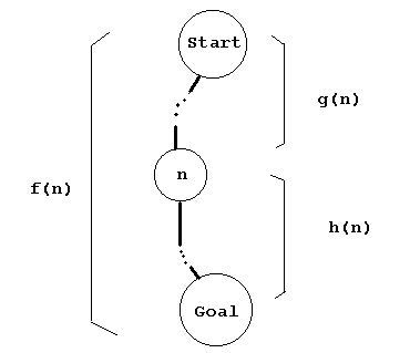
Fig. 5.1
Section 2.16 introduced an outline for a simple Prolog search program. This section discusses heuristic search using the A* algorithm, due to Nilsson (1980).
Heuristic search uses a heuristic function to help guide the search. When a node is expanded, each of its children is evaluated using a search function. Each child is placed into a list of nodes -- the so-called open list -- in order determined by the search function evaluation (smaller values first). The heuristic function estimates how much work must be done to reach a goal from the node in question. Typically, the search function f is expressed as

Here is some simple pseudocode from which the Prolog program will be
developed.
When a goal has been reached, one would certainly like to be able to return the solution path from the start to the goal. The pseudocode ignored this feature, but it will be included as the Prolog prototype program is developed.
A common cost function g(-) is path length. The cost of getting from the start node to a current node is the length of relevant path. This can be computed incrementally, as will be seen.
It is important to realize that this kind of search can follow a contiguous path for a while, until some previously unchosen node n has the current smallest f(-) value, in which case this node n is expanded, and its children considered.
Now for the Prolog program for the A* search.
Let us assume that State refers to some description of the state of a search. For example State might be a description of the 8-puzzle tile for a specific configuration, as developed in the next section. A Node in the search space (or graph) needs to record the State, the Depth (or path length from the start), the value of f(-) for the node F, and a list of the ancestors A of this node. We will use the Prolog term structure
In general, if the Depth is replace by some other cost, the node representation would be similar; just replace Depth by a cost, and compute it appropriately. Also, we will see in the next section (8-puzzle) that the ancestor list might be more conveniently saved as a list of symbolic actions (used to achieve successive states), rather that as a list of the actual full nodes themselves. Other modifications of the prototypical A* algorithm presented in this section might be made, depending on the application.
The main predicate for the program is
solve(Start,Soln) :- f_function(Start,0,F),
                     search([Start#0#F#[]],S),
                     reverse(S,Soln).

f_function(State,D,F) :- h_function(State,H),
                         F is D + H.
The 'Start' variable refers to the starting state description. The first
parameter for the search
predicate represents the open list. The 'h_function'
definition needs to be supplied with the particular application.
search([State#_#_#Soln | _], Soln) :- goal(State).
search([B|R],S) :- expand(B, Children),
                   insert_all(Children, R, NewOpen),
                   search(NewOpen,S).
The version of the 'expand' predicate given here simply uses Prolog's
bagof computation (thus bundling up a lot of work).
expand(State#D#_#A, All_My_Children) :-
         bagof(Child#D1#F#[Move|A],
               ( D1 is D + 1,
                 move(State,Child,Move),
                 f_function(Child,D1,F) ) ,
               All_My_Children).
The (application dependent) 'move' predicate should generate the 'Child' states, in such a way as to obtain them all by backtracking. (See the 8-puzzle example in the next section.) As previously stated, the 'Move' can either be the the whole parent node itself or some appropriate substitute. (Actually, one should rewrite the 'expand' clause if one is going to use the whole node, rather some symbolic representation, as we do in the next section.)
Here is the code for insert_all. It is a familiar kind of insertion-sort algorithm ...
insert_all([F|R],Open1,Open3) :- insert(F,Open1,Open2),
                                 insert_all(R,Open2,Open3).
insert_all([],Open,Open).

insert(B,Open,Open) :- repeat_node(B,Open), ! .
insert(B,[C|R],[B,C|R]) :- cheaper(B,C), ! .
insert(B,[B1|R],[B1|S]) :- insert(B,R,S), !.
insert(B,[],[B]).

repeat_node(P#_#_#_, [P#_#_#_|_]).

cheaper( _#_#H1#_ , _#_#H2#_ ) :- H1 <  H2.
The following exercises ask the reader to formulate A* solutions to various problems or puzzles. See the next section, 5.2 on the 8-puzzle, as an example of how to extend the general A* program of this section to a specific solution of the 8-puzzle.
Exercise 5.1.1 Formulate an A* algorithm for the N queens puzzle. (See section 2.11 for a simple, but inefficient, approach.)
Exercise 5.1.2 Formulate an A* approach to maze solving.