Fig. 3.3.1
Chapter 6 studies some prolog meta-interpreters for logic.
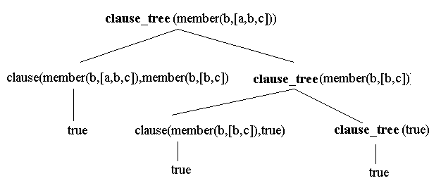
The following program specifies an interpreter of clause trees in Prolog
To illustrate how this meta-interpreter works, let us use it to interpret the program for 'member':clause_tree(true) :- !. /* true leaf */ clause_tree((G,R)) :- !, clause_tree(G), clause_tree(R). /* search each branch */ clause_tree(G) :- clause(G,Body), clause_tree(Body). /* grow branches */
Consider the goalmember(X,[X|_]). member(X,[_|R]) :- member(X,R).
So the meta-interpreter grows clause trees, and finds the same answers that Prolog itself would calculate. Here is a program clause tree rooted at 'clause_tree(membr(b,[a,b,c]))':?- clause_tree(member(X,[a,b,c]). X = a ; X = b ; X = c ; no
One can add evaluation to the 'clause_tree' program. The way this is done depends upon the kind of Prolog one is using.
clause_tree(true) :- !.
clause_tree((G,R)) :-
   !,
   clause_tree(G),
   clause_tree(R).
clause_tree(G) :-
   (predicate_property(G,built_in) ;
     predicate_property(G,compiled) ),
   call(G).              %% let Prolog do it
clause_tree(G) :- clause(G,Body), clause_tree(Body).
The new third clause says that if the goal G is built_in (e.g., arithmetic) then call the
underlying Prolog goal to do the evaluation; and similarly if G is compiled into memory.
So, for example, with the new definition
?- clause_tree((X is 3, X <  5)).
X = 3
Meta-interpreters are very useful for redesigning the control mechanisms of Prolog. For example, consider the following program:
If one were to try the Prolog goal ?- p the first two clauses would be the cause of infinite looping, like in the following derivationp :- q. q :- p. p :- r. r.
However, it is still a very interesting problem to try to detect some loops. Here is a modification of the 'clause_tree/1' program that can detect some loops:
We have added a Trail parameter to the meta-interpreter, and a 'loop_detect'. It is instructive to compare this program with the search program in section 2.13. Now, we haveclause_tree(true,_) :- !. clause_tree((G,R),Trail) :- !, clause_tree(G,Trail), clause_tree(R,Trail). clause_tree(G,Trail) :- loop_detect(G,Trail), !, fail. clause_tree(G,Trail) :- clause(G,Body), clause_tree(Body,[G|Trail]). loop_detect(G,[G1,_]) :- G == G1. loop_detect(G,[_,R]) :- loop_detect(G,R).
The third clause "catches" the loop and allows the other choice 'p :- r' to be tried.?- clause_tree(p,[]). yes
Now consider the following modification of the program. This version also generates a clause tree parameter value as it interprets a program.
clause_tree(true,_,true) :- !.
clause_tree((G,R),Trail,(TG,TR)) :-
   !,
   clause_tree(G,Trail,TG),
   clause_tree(R,Trail,TR).
clause_tree(G,_,prolog(G)) :-
   (predicate_property(G,built_in) ;
     predicate_property(G,compiled) ),
   call(G).              %% let Prolog do it
clause_tree(G,Trail,_) :-
   loop_detect(G,Trail),
   !,
   fail.
clause_tree(G,Trail,tree(G,T)) :-
   clause(G,Body),
   clause_tree(Body,[G|Trail],T).
Load both this last program and the simple test program
and then issue the following goal ...p(X) :- q(X), r(Y), X < Y. q(3). r(2). r(5). r(10).
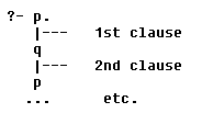
Here is a program to draw the clause tree that is generated ...?- clause_tree(p(X),[],Tree) Tree = tree(p(3),(tree(q(3),true),tree(r(5),true),prolog(3 < 5))) X = 3 ; Tree = tree(p(3),(tree(q(3),true),tree(r(10),true),prolog(3 < 10))) X = 3 ; No
why(G) :- clause_tree(G,[],T),
          nl,
          draw_tree(T,5).

draw_tree(tree(Root,Branches),Tab) :- !,
   tab(Tab),
   write('|-- '),
   write(Root),
   nl,
   Tab5 is Tab + 5,
   draw_tree(Branches,Tab5).
draw_tree((B,Bs),Tab) :- !,
   draw_tree(B,Tab),
   draw_tree(Bs,Tab).
draw_tree(Node,Tab) :-
   tab(Tab),
   write('|-- '),
   write(Node),
   nl.
Now, interpreting the same sample program as above ...
?- why(p(X)).

   |-- p(3)
        |-- q(3)
             |-- true
        |-- r(5)
             |-- true
        |-- prolog(3 <  5)

X = 3 ;

   |-- p(3)
        |-- q(3)
             |-- true
        |-- r(10)
             |-- true
        |-- prolog(3 <  10)

X = 3 ;

No
The tree corresponding to the first answer would be drawn ("vertically oriented") as
follows... 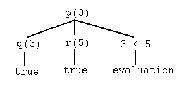
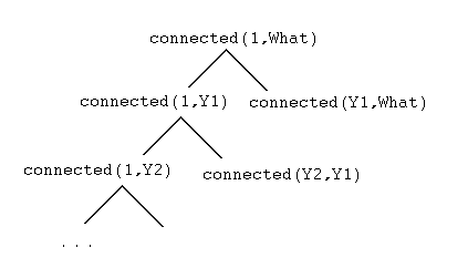
To motivate the last topic in this section, consider the following "bad" program
If one were to try to compute 'connected' using Prolog, there is going to be a problem with "left recursion". For example,connected(X,Y) :- connected(X,Z), connected(Z,Y). connected(1,2). connected(2,3). connected(3,4). connected(4,5).
This goal causes Prolog to go into an infinite subgoal descent. (Try this yourself!) Of course, we could have prevented this -- for this goal -- if we had put the "rule" after the "facts" in the bad program. But, even with that change, a goal like '?- connected(1,What)' would have caused a problem if we forced backtracking to try to find all solutions. (Again, try this yourself.)?- connected(1,2). ...
The looping here
is not like the looping discussed above. To explain this, consider the original "bad"
program, and consider the Prolog derivation tree generated by attempting the goal
'?- connected(1,What)'
One method for avoiding this kind of infinite descent is called "iterative deepening", which means that one still uses depth-first search, but one "iteratively" searches to a certain depth, then deeper, then deeper still, ..., etc. Here is a meta-interpreter that does this. This meta-interpreter is quite similar to the previous ones. However, this one has only two extra parameters: one for current depth of a goal, and one for the current depth limit. This interpreter does not do the previous kind of loop check nor does it generate the symbolic tree, but it does call Prolog for evaluation goals. (Of course, these features could be easily added, but here we concentrate just on the iterative deepening concept.)
clause_tree(true,_,_) :- !.
clause_tree(_,D,Limit) :- D > Limit,
                          !,
                          fail.  %% reached depth limit
clause_tree((A,B),D,Limit) :- !,
                              clause_tree(A,D,Limit),
                              clause_tree(B,D,Limit).
clause_tree(A,_,_) :- predicate_property(A,built_in),
                      !,
                      call(A).
clause_tree(A,D,Limit) :- clause(A,B),
                          D1 is D+1,
                          clause_tree(B,D1,Limit).

iterative_deepening(G,D) :- clause_tree(G,0,D).
iterative_deepening(G,D) :- write('limit='),
                            write(D),
                            write('(Hit Enter to Continue.)'),
                            get0(C),
                            ( C == 10 ->
                                 D1 is D + 5,
                                 iterative_deepening(G,D1)  ).
Note that the intended interpreter is 'iterative_deepening(+Goal,+InitDepth)' where
+Goal could, of course, contain variables. This iterative deepening meta-interpreter
uses "stages": the depth of the first stage is +InitDepth, the second stage goes to
depth InitDepth+5, etc.
So now, suppose that this program and the original 'connected' program have been loaded. What happens this time? ...
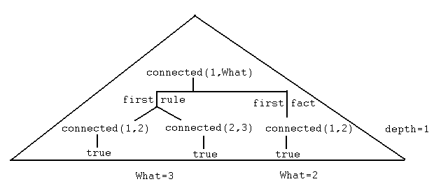
Note how the 'iterative_deepening' meta-interpreter finds solutions first that are near the current depth limit, and then proceeds to discover shallower solutions. A good graphical description of this phenomenon is that the meta-interpreter searches the lower left corner of a triangle of depth equal to the current depth limit and then searches shallower depths in the right portion of the triangle, as suggested by the following diagram. The diagram shows solutions for connected(1,What) that are "accessible" at depth 1, which was the first stage for the goal above.?- iterative_deepening(connected(1,What), 1). What=3 ; What=2 ; Limit=1(Hit Enter to Continue) What=5 ; What=5 ; What=5 ; What=4 ; What=5 ; What=5 ; What=4 ; What=3 ; What=2 ; Limit=6(Hit Enter to Continue.) What=5 %% stop Yes
Exercise 3.3.2 Consider the program
p(a) :- p(X).
p(b).
Show that 'clause_tree/2' above will not detect the loop for this program. Can you redesign the loop-check so that the looping in this example will be stopped?
The second exercise shows that it can be difficult to detect particular kinds of loops (aside from the impossibility of detecting all loops).
Exercise 3.3.3 The meta-interpreter 'clause_tree' grows program clause trees. It does not (exactly) model Prolog derivation trees! Explain why. Hint: Note that Prolog derivation trees have nodes which are sequences of literals. Design a Prolog meta-interpreter, similar to the one at the beginning of this section, but one whose nodes are sequences of subgoals. Is this new interpreter equivalent to the one in this section? (Define what equivalent would mean first.) Implement loop checking for this meta-interpreter.