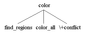
Fig. 2.9
This section reconsiders the map coloring problem from Section 2.1. This time we shall represent the adjacent regions using a list of neighboring regions, and not necessarily store the map explicitly using data in the program. For example, the map in Section 2.1 could be represented with the following adjacency list representation
[[1,2],[1,3],[1,4],[1,5],[2,3],[2,4],[3,4],[4,5]]
The intention is to design a coloring program that could be used as follows:
?- color([[1,2],[1,3],[1,4],[1,5],[2,3],[2,4],[3,4],[4,5]],
                  [red,green,blue,yellow],Coloring).
Coloring = [[5,red],[4,green],[3,red],[1,blue],[2,yellow]] ; ...   /* 48 solutions */
Notice that here, for example, 1 and 3 are adjacent because [1,3] belongs to the list, but 3 is adjacent to 1 for the same reason. We can compute the adjacency relation generally using the following definition.
adjacent(X,Y,Map) :- member([X,Y],Map) ; member([Y,X],Map).
Note the disjunction, ';', in the clause. X and Y represent names of regions and Map is an adjacency list. The predicate 'member' was defined in the last section, 2.7.
Notice that an adjacency list can be used to define the map as long as every region is adjacent to at least one other region (not disconnected regions). So one can compute a list of region names, given the adjacency list. Here is a Prolog definition for this.
find_regions([],R,R).
find_regions([[X,Y]|S], R,A) :-
     (member(X,R) ->
        (member(Y,R) -> find_regions(S,R,A) ; find_regions(S,[Y|R],A)) ;
           (member(Y,R) -> find_regions(S,[X|R],A) ; find_regions(S,[X,Y|R],A) ) ).
This is the most complicated Prolog implication form so far. Spend some time understanding what it says before going on. For example,
?- find_regions([[1,2],[1,3],[1,4],[1,5],[2,3],[2,4],[3,4],[4,5]],[],R).
R = [5,4,3,1,2]
Pay particular attention to the use of the accumulating parameter (the second parameter).
Now, given the adjacency list and a list of colors, one should be able to compute proper colorings -- that is, colorings where adjacent regions have different colors. In words, stated in a top-down fashion, the intention is to color the map by means of first calculating the regions from the adjacency list, then color the map, then check to see that the coloring is not in conflict. Pictured with a tree, we have

The tree shows the intended top-down logical decomposition for the program design. Later, with values filled in for variables, it could become a clause tree justifying some particular consequence of the program.
color(Map,Colors,Coloring) :-
        find_regions(Map,[],Regions),
        color_all(Regions,Colors,Coloring),
        \+ conflict(Map,Coloring).

color_all([R|Rs],Colors,[[R,C]|A]) :-
        member(C,Colors),
        color_all(Rs,Colors,A).
color_all([],_,[]).


conflict(Map,Coloring) :-
        member([R1,C],Coloring),
        member([R2,C],Coloring),
        adjacent(R1,R2,Map).
It is very important to realize where the running program makes choices for colorings. Basically, this happens in the first defining clause for 'color_all', and the choices are determined by 'member'. Backtracking on 'member', chooses another color.
Exercise 2.9 The program is somewhat inefficient in that it waits until after it has completely colored a map before it determines whether there is a conflict in the coloring. Modify the program so that its colors and checks against conflict simultaneously (before continuing to color more regions). Test the modified and the original program on a map of the United States.