|
Computer Science Department California State Polytechnic University Pomona, California, USA jrfisher@csupomona.edu |
Department of Computer Science University of Bergen Bergen, Norway bezem@ii.uib.no |
Geolog is a logic programming language for finitary geometric logic. These webnotes describe how to use a Geolog interpreter written in Prolog, called Geoprolog. These notes also provide examples showing how to prove some interesting mathematical theorems using Geoprolog. Another section (§8) discusses an interactive version of the software that connects a Prolog prover with a Java GUI.
The authors have developed machine models for describing Geolog computations. An interesting approach involves what we call Skolem Machines. A Skolem machine is another abstract model for computation. Skolem machines have Geolog theories as input instructions. Skolem machines have computational power generally equivalent to Turing Machines. Click on the link for §0 below to read a short article regarding some basic definitions of the Geolog language and Skolem machine operations. The references at the end of the article cite theoretical work. Skolem machines (as formulated by us) are named after the eminent Norwegian mathematician and logician Thoralf Skolem (1887-1963). Historically, the essential ideas behind Skolem Machines were "invented" by Thoralf Skolem about 87 years ago!!! See our notes in §0, which briefly explains this connection. A nice biography of T.Skolem is posted here.
If one clicks on the "SM" links, a proof demonstration Java applet opens in a new window. The resulting interactive display simulates a Skolem machine computation, in tree form, for the corresponding theory. The interaction is NOT computing the tree: It is displaying the tree inferences generated by the iG program described in §8.
For example, click here: SM to see a sample Skolem machine computation for the little theory described in the whitepaper of §0.
If you would like to make comments or ask questions about this website please email us (links above).
Note added October 2008: An experimental portable Java application implementing Geolog is available at the link GeologUI.
§0. Technical Notes on the Geolog language and Skolem Machines (pdf)
§1. download some files
§2. start Prolog and load geoprolog.pl
§3. working with Geolog theories
§4. writing Geolog rules
§5. working with "runaway" theories
§6. Sample Geolog theories and proofs6a- dpe Diamond Property in rewriting theory SM§7. minimal case proofs
6b- latt_assoc & latt_comm associativity and commutativity of the supremum operation in a lattice
6c- nl Newman's Lemma in rewriting theory
6d- p1p2 & p2p1 side conditions in Pappus' Theorem in plane geometry
6e- mb transitive relations property
6f- unf confluence of a rewrite relation implies uniqueness of normal forms
6g- r3_5 Ramsey number COUNTERMODEL, 3-cliques on 5 points SM
§8. interactive Geolog proof browser
The Prolog source code file geoprolog.pl (~8KB).Create a directory called "geolog" on your system and move these files into that directory, as shown in the following diagram.
The Java tree visualizer GeologTree.jar (~20KB).
The sample Geolog theory source file dpe.gl (~4KB), example for § 3.
The sample Geolog theory source file inf.gl (~4KB), example for § 6.
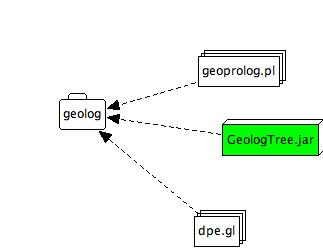
Additional files to download will be linked, as needed, in later sections.
/opt/local/bin/swipl -L0 -G0 -f geoprolog.pl -g trueThis will initialize SWI-Prolog and load the GeoProlog interpreter ...
_^_%%%%%%%%%%%%%%%%%%%%%%%%%%%%%%%%%%%%%%%%%%%%%%%%% 03/01/2007 %% GeoProlog %% ?- compile(+G). % Compile Geolog rules in file G.gl %% ?- show. % Show ordered rules ... %% ?- go. % Attempt proof ... %% Control C stops runaway 'go'... hit 'a' key for abort %% ?- golog. % go+log if 'go' terminated %% ?- golog(+N). % go+log, N steps only %% ?- tree. % Show search tree for last golog ... %% ?- proof. % Generate minimal case proofs ... %% ?- info. % Display this info %%%%%%%%%%%%%%%%%%%%%%%%%%%%%%%%%%%%%%%%%%%%%%%%%%%%%%%%%%%%%%%% % /geolog/geoprolog/geoprolog.pl compiled 0.00 sec, 20,848 bytes ?-
The geoprolog goal compile(+G) loads the file G.gl and compiles it into internal Prolog code (and shows the rules after compiling).?- compile(dpe). true=>exists(a), exists(b), exists(c) re(b, _G305), re(c, _G305)=>goal exists(_G304)=>e(_G304, _G304) true=>re(a, b), re(a, c) e(_G304, _G305)=>e(_G305, _G304) e(_G304, _G305), re(_G305, _G308)=>re(_G304, _G308) e(_G304, _G305)=>re(_G304, _G305) r(_G304, _G305)=>re(_G304, _G305) re(_G304, _G305)=>e(_G304, _G305);r(_G304, _G305) r(_G304, _G305), r(_G304, _G308)=>_G363^ (exists(_G363), r(_G305, _G363), r(_G308, _G363)) dpe.gl compiled to prolog. Yes ?-
The geoprolog goal show can be used to list the ordered Geolog rules, after compiling them. These rules are residing in Prolog memory for use.
The geoprolog goal go attempts to prove the theory residing in Prolog memory.
It took about 0.00 seconds (negligible time) on our system to prove the theory, and the proof required 9,994 Prolog inferences.?- go. % 11,419 inferences, 0.01 CPU in 0.00 seconds (216% CPU, 1141900 Lips) Yes ?-
The geoprolog prover could prove the theory in the loaded file unf.gl. To see a visual proof, use first the goal golog and then goal diagram, or combine them as follows ...
At this point a proof is generated and then displayed in a separate window ...?- golog, tree. %% gl/dpe.log created WAIT FOR geologTree TO START ...
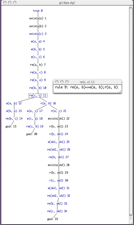
This display is the Java program (geologTree.jar) running and displaying the derivation generated by geoprolog. Each branch of the tree represents a state generated during the geoprolog search process.
The scale of the tree was reduced. Right-click on the background of the tree panel and the following popup menu will appear

One can select nodes (facts) in the tree by clicking on them. The selected node is outlined and a separate window shows the inferences relevant to the selected node. This is illustrated in the previous display.
When the Java window is dismissed, the Prolog process again gets the focus.
Your system needs to be able to run Java jar files, in order to display geolog trees.
The geologTree.jar program can be started separately by double-clicking on its icon at any time. The user can then drag any "--.dgl" file (previously created by geoprolog) and drop it on the geologTree panel, and then the panel will display the corresponding tree.
If, for other inputs, geoprolog halts with a counter-example, then the diagram goal will give a visual representation of how the counter-example was generated. Branches of the resulting tree not terminating with 'goal' or 'false' represent counter-models (states).
Section 7 explains the '?- proof.' goal.
Geolog rules have the form
The part on the left-hand-side of => is called the antecedent of the rule, and the right-hand-side is called the consequent. The antecedent is a conjunction of atomic Prolog terms (separated by ","). The consequent is a disjunction (separated by ";"). Each disjunt Cj is itself a conjunction, having form
where each Bj is an atomic Prolog term.
The atomic terms Ai and Bj can contain variables. The variables appearing in the entecedant are universal variables whose scope is the entire rule. Universal variables can occur anywhere in the entire rule. Variables appearing in some Cj which are not universal are called existential variables and their scope is only the particular disjunct Cj in which they appear.
The universal and existential terminology refers to first-order predicate logic. Universal variables are universally quantified (implicitly) and existential variables are exitentially quantified (implicitly).
There are three special rule forms: factuals, goal rules, and false rules,
true => C1 ; C2; ... ; Cn .Example 1.
A1, A2, ..., Am => goal .
A1, A2, ..., Am => false .
The Geolog rule: p(X) => q(Y),s(X,Y) ; r(Z).Example 2.Internal geoprolog form: p(_G310)=>_G352^ (q(_G352), s(_G310, _G352));_G381^r(_G381)
1st-order logic: ∀(X){p(X) ⇒ ∃(Y)[q(Y) ∧ s(X,Y)] ∨ ∃(Z)r(Z)}
The Geolog rule: p(X) => q(Y),s(X,Y) ; r(Y).Notice that the Geolog rule in Example 2 is only slightly different that the Geolog rule in Example 1: The last variable is "Y" in Example 2 rather than "Z" as in Example 1. However, the scope of the last "Y" is only the last disjunct, as shown in the 1st-order logic forms. The geoprolog loader transcribes rules to be consistent with the intended logical form by automatically renaming the existential variables in the disjuncts of the consequent of the rule.Internal geoprolog rule form: p(_G310)=>_G352^ (q(_G352), s(_G310, _G352));_G381^r(_G381)
1st-order logic: ∀(X){p(X) ⇒ ∃(Y)[q(Y) ∧ s(X,Y)] ∨ ∃(Y)r(Y)}
The programmer can count on this renaming to be automatically performed for all rule inputs. The scope of an existential variable in the consequent of any rule will automatically be restricted to the particular disjunct in which it occurs.
In order to express that an entity should belong to the domain of a Geolog theory, the user can reserve a special predicate for this purpose. In the following theory, for example, the predicate 'domain' is used for this purpose. The user chooses the specific name for the domain closure predicate. The names 'domain' or 'exists' are recommended because they suggest the role that the predicate plays in the theory.
Example 3.
The Geolog theory:Internal geoprolog rule forms:true => domain(X), p(X). % #1 p(X) => q(X) ; r(X) ; domain(Y), s(X,Y). % #2 domain(X) => u(X). % #3 u(X), q(X) => false. % #4 r(X) => goal. % #5 s(X,Y) => goal. % #61st-order logic forms:true=>_G348^ (domain(_G348), p(_G348)). p(_G323)=>q(_G323);r(_G323);_G407^ (domain(_G407), s(_G323, _G407)). domain(_G323)=>u(_G323). u(_G323), q(_G323)=>false. r(_G323)=>goal. s(_G323, _G324)=>goal.true => ∃(X)[domain(X) ∧ p(X)]
∀(X){p(X) ⇒ ∃(Y)[q(Y) ∧ s(X,Y)] ∨ ∃(Z)r(Z)}
∀(X)[domain(X) => u(X)]
∀(X)[u(X) ∧ q(X) => false]
∀(X)[r(X) => goal]
∀(X)∀(Y)[s(X,Y) => goal]
The second rule introduces a function symbol, in addition to being a splitting rule. If the second and third rules were to be interchanged, the goal would be easily supported, using geoprolog. (Try this!)true => p(a). p(X) => p(f(X)) ; q(X). p(f(a)) => goal. q(X) => goal.
However, as is, the second rule introduces recursive attempts to satisfy p(-). The illustration in this section demonstrates how to control a "runaway" search and how to inspect what it is that the runaway search was generating.
Assume that geoprolog.pl is loaded and running (see §2) . The following SWI-Prolog interactions illustrate what might happen...
?- compile(inf).
true=>p(a).
p(_G325)=>p(f(_G325));q(_G325).
p(f(a))=>goal.
q(_G325)=>goal.
%% gl/inf.gl compiled to Prolog.

Yes
?- go.
^C
Action (h for help) ? abort
% 1,815,948 inferences, 2.53 CPU in 3.97 seconds (64% CPU, 717766 Lips)
% Execution Aborted

?- golog(5), tree.
%% gl/inf.log created
WAIT FOR geologTree TO START ...
            %% The diagram is displayed ... and then dismissed ...
Yes
Here is the diagram that was displayed after the Prolog command
golog(5), diagram in the previous interaction ...
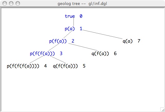
The diagram shows a pattern of incomplete inference (stopping at level 5). Notice that the second rule repeatedly applies and splits.
If one clicks on the "SM" links, a proof demonstration applet opens in a new window. The resulting interactive display simulates a Skolem machine computation, in tree form, for the corresponding theory. The interaction is NOT computing the tree, rather it is displaying the inferences generated by the iG program described in §8.
In particular, click here: SM to see a sample Skolem machine computation for the little theory described in the whitepaper of §0.
The Diamond Property (DP) in rewriting theory states that, if x rewrites to both y and z, then the latter two rewrite both to some u (all in one step). We prove that if some rewrite relation satisfies DP, then its reflexive closure also satisfies DP (reflexive closure means adding point loops to every point).The first theory input displayed above is M. Bezem's original input form. When a file of this form (.in file extension) is read by the Geoprolog system it automatically converts it to Geolog form (displayed in the second listing above). Geoprolog reads dpe.in, translates to Geolog form and writes file dpe.gl, and then loads and compiles the Geolog version. The annotations in the original (.in) file explain the role of each rule. The converted file (.gl) does have the corresponding annotation written as a comment before the Geolog rule.In the following code e is equality, r the rewrite relation, and re = r + e (that is, the reflexive closure of r).
% dpe.in
% DP(r) => DP(re), i.e.,
% the diamond property is preserved under reflexive closure

name(dpe).

:- dynamic e/2,r/2,re/2.

% domain elements a,b,c
dom(a). dom(b). dom(c).

_ axiom assumption              : (true => re(a,b),re(a,c)).
_ axiom goal_axiom(X)           : (re(b,X),re(c,X) => goal).

% equality axioms
_ axiom reflexivity_of_e(X)     : (dom(X) => e(X,X)).
_ axiom symmetry_of_e(X,Y)      : (e(X,Y) => e(Y,X)).
_ axiom left_congr_of_e(X,Y,Z)  : (e(X,Y),re(Y,Z) => re(X,Z)).

% basic facts on re
_ axiom re_contains_e(X,Y)      : (e(X,Y) => re(X,Y)).
_ axiom re_contains_r(X,Y)      : (r(X,Y) => re(X,Y)).
_ axiom re_elimination(X,Y)     : (re(X,Y) => e(X,Y);r(X,Y)).

% DP
_ axiom diam_prop_of_r(X,Y,Z)   : (r(X,Y),r(X,Z) => dom(U),r(Y,U),r(Z,U)).
%% Converted from dpe.in

%% domain declaration
true=>dom(a).

%% domain declaration
true=>dom(b).

%% domain declaration
true=>dom(c).

%% _G304 axiom assumption
true=>re(a, b), re(a, c).

%% _G306 axiom goal_axiom(_G289)
re(b, _G289), re(c, _G289)=>goal.

%% _G302 axiom reflexivity_of_e(_G289)
dom(_G289)=>e(_G289, _G289).

%% _G304 axiom symmetry_of_e(_G289, _G290)
e(_G289, _G290)=>e(_G290, _G289).

%% _G311 axiom left_congr_of_e(_G289, _G290, _G291)
e(_G289, _G290), re(_G290, _G291)=>re(_G289, _G291).

%% _G304 axiom re_contains_e(_G289, _G290)
e(_G289, _G290)=>re(_G289, _G290).

%% _G304 axiom re_contains_r(_G289, _G290)
r(_G289, _G290)=>re(_G289, _G290).

%% _G310 axiom re_elimination(_G289, _G290)
re(_G289, _G290)=>e(_G289, _G290);r(_G289, _G290).

%% _G322 axiom diam_prop_of_r(_G289, _G290, _G291)
r(_G289, _G290), r(_G289, _G291)=>dom(_G302), r(_G290, _G302), r(_G291, _G302).
?- compile('in/dpe').
%% in/dpe.in converted to in/dpe.gl
true=>dom(a). %1
true=>dom(b). %2
true=>dom(c). %3
true=>re(a, b), re(a, c). %4
re(b, _G360), re(c, _G360)=>goal. %5
dom(_G359)=>e(_G359, _G359). %6
e(_G359, _G360)=>e(_G360, _G359). %7
e(_G359, _G360), re(_G360, _G363)=>re(_G359, _G363). %8
e(_G359, _G360)=>re(_G359, _G360). %9
r(_G359, _G360)=>re(_G359, _G360). %10
re(_G359, _G360)=>e(_G359, _G360);r(_G359, _G360). %11
r(_G359, _G360), r(_G359, _G363)=>_G481^ (dom(_G481), r(_G360, _G481), r(_G363, _G481)). %12
%% in/dpe.gl compiled to Prolog.
Yes
At the present time there is
no "official" way to annotate Geolog rules, other than using comments.
However, the authors do intend to allow for annotations of rules that
can appear as appropriately instantiated annotations in proofs in future versions.
The sample execution in §3 shows the proof tree generated by Geoprolog.
These two prove associativity and commutativity of the supremum operation in a lattice. The formalization is a bit special as the supremum is defined as a ternary relation and equality is defined by x=y iff x<=y and y<=x.Exercise: Download each of these files, load each of them (separate sessions) into Geoprolog and diagram the proofs.% latt_asssoc.in :- dynamic lt/2,j/3. name(l). dom(x). dom(y). dom(u). dom(z). dom(v). dom(w). _ axiom assump : (true => j(x,y,u),j(u,z,v),j(y,z,w)). _ axiom goal_ax : (j(x,w,V),lt(v,V),lt(V,v) => goal). _ axiom lt_refl(X) : (dom(X) => lt(X,X)). _ axiom lt_trans(X,Y,Z) : (lt(X,Y),lt(Y,Z) => lt(X,Z)). _ axiom ub_join(X,Y,Z) : (j(X,Y,Z) => lt(X,Z),lt(Y,Z)). _ axiom lub_join(X,Y,Z,U) : (j(X,Y,Z),lt(X,U),lt(Y,U) => lt(Z,U)). _ axiom lt_j(X,Y) : (lt(X,Y) => j(X,Y,Y)). _ axiom commute_j(X,Y,Z) : (j(X,Y,Z) => j(Y,X,Z)). _ axiom up_latt(X,Y) : (dom(X),dom(Y) => dom(U),j(X,Y,U)).
% latt_comm.in
:- dynamic lt/2,j/3.

name(l_c).

dom(x). dom(y). dom(z).

_ axiom assump : (true => j(x,y,z)).
_ axiom goal_ax  : (j(y,x,Z),lt(z,Z),lt(Z,z) => goal).

_ axiom lt_refl(X) : (dom(X) => lt(X,X)).
_ axiom lt_trans(X,Y,Z) : (lt(X,Y),lt(Y,Z) => lt(X,Z)).
_ axiom ub_join(X,Y,Z) : (j(X,Y,Z) => lt(X,Z),lt(Y,Z)).
_ axiom lub_join(X,Y,Z,U) : (j(X,Y,Z),lt(X,U),lt(Y,U) => lt(Z,U)).
_ axiom lt_j(X,Y) : (lt(X,Y) => j(X,Y,Y)).
_ axiom up_latt(X,Y) : (dom(X),dom(Y) => dom(U),j(X,Y,U)).
Newman's Lemma in rewriting theory states that a rewrite relation is confluent if it is terminating and locally confluent. Huet's proof is by well-founded induction. We prove the induction step in this proof.Exercise: Download nl.in, load it into Geoprolog and diagram the proof.% nl.in % induction step in Newman's Lemma name(nl). :- dynamic e/2,r/2,s/2. %domain elements a,b,c dom(a). dom(b). dom(c). _ axiom found(X) :(s(b,X),s(c,X) => goal). _ axiom assump :(true => s(a,b),s(a,c)). _ axiom ref_e(X) :(dom(X) => e(X,X)). _ axiom sym_e(X,Y) :(e(X,Y) => e(Y,X)). _ axiom e_in_s(X,Y) :(e(X,Y) => s(X,Y)). _ axiom r_in_s(X,Y) :(r(X,Y) => s(X,Y)). _ axiom trans_s(X,Y,Z) :(s(X,Y),s(Y,Z) => s(X,Z)). _ axiom lo_cfl(X,Y,Z) :(r(X,Y),r(X,Z) => dom(U),s(Y,U),s(Z,U)). _ axiom ih_cfl(X,Y,Z) :(r(a,X),s(X,Y),s(X,Z) => dom(U),s(Y,U),s(Z,U)). % last to avoid infinite path _ axiom e_or_rs(X,Y) :(s(X,Y) => e(X,Y);dom(Z),r(X,Z),s(Z,Y)).
The side conditions in Pappus' Theorem in plane geometry can be rather different. Pappus1 is with side condition: the 3 points on one line are not the other and conversely. Pappus2 is with side condition that the pairs of crossing lines have unique intersections (that is, pairs of different lines). We prove that Pappus1 implies Pappus2 (p1p2) and the converse (p2p1).The p1p2 theory has a long proof. Click here to see a schematic image of the proof tree (opens in separate window). The snapshot was obtained using GeologTree along with scale reduction (right-click on panel, choose "smaller" ...). The scale reduction on this snapshot is so great that the nodes to do not appear. The purpose of the snapshot is to display the complexity of the proof. One can examine the proof at normal scales. We also use this example to illustrate the extraction of minimal case proofs in the next section. Notice that many of the cases have similar "shapes". (Are they the same?)Pappus1 is with sidecondition: the 3 points on one line are not the other and conversely. Pappus2 is with sidecondition that the pairs of crossing lines have unique intersections (that is, pairs of different lines).
% p1p2.in
% Pappus1 => Pappus2 in projective planes

name(p1p2_).

:- dynamic ep/2,el/2,pl/2,col/4.
%ep,el = equality for points and lines, resp.
%pl = point-line incidence (deliberately asymmetric!)
%col = point-point-point-line collinearity

%points
dom(a). dom(b). dom(c). dom(d). dom(e). dom(f). dom(g). dom(h). dom(i).
%lines
dom(l). dom(m). dom(n). dom(o). dom(p). dom(q). dom(r). dom(s).

%Pappus2 assumptions, same as in Pappus1
_ axiom assump1 : (true => col(a,b,c,l),col(d,e,f,m)). %a,b,c on l, etc.
_ axiom assump2 : (true => col(b,f,g,n),col(c,e,g,o)).
_ axiom assump3 : (true => col(b,d,h,p),col(a,e,h,q)).
_ axiom assump4 : (true => col(c,d,i,r),col(a,f,i,s)).

%Pappus2 conclusions
_ axiom goal1    : (el(n,o) => goal).
_ axiom goal2    : (el(p,q) => goal).
_ axiom goal3    : (el(s,r) => goal).
_ axiom goal4(U) : (el(U,U),pl(g,U),pl(h,U),pl(i,U) => goal).
%not using col(g,h,i,U) for efficiency reasons ...

%collinearity, we avoid the symmetries inflicted by col_intro
_ axiom col_elim1(P,Q,R,L) : (col(P,Q,R,L) => pl(P,L)).
_ axiom col_elim2(P,Q,R,L) : (col(P,Q,R,L) => pl(Q,L)).
_ axiom col_elim3(P,Q,R,L) : (col(P,Q,R,L) => pl(R,L)).
% axiom col_intro(P,Q,R,L) : (pl(P,L),pl(Q,L),pl(R,L) => col(P,Q,R,L)).

%equality for points
_ axiom pref(P,L)   :  (pl(P,L) => ep(P,P)).     %a bit special indeed!
_ axiom psym(P,Q)   :  (ep(P,Q) => ep(Q,P)).
_ axiom ptra(P,Q,R) :  (ep(P,Q),ep(Q,R) => ep(P,R)).

%equality for lines
_ axiom lref(P,L)   :  (pl(P,L) => el(L,L)).     %a bit special indeed!
_ axiom lsym(L,M)   :  (el(L,M) => el(M,L)).
_ axiom ltra(L,M,N) :  (el(L,M),el(M,N) => el(L,N)).

%congruence
_ axiom pcon(P,Q,L) :  (ep(P,Q),pl(Q,L) => pl(P,L)).
_ axiom lcon(P,L,M) :  (pl(P,L),el(L,M) => pl(P,M)).

%Pappus1: A,B,C on L not on M, D,E,F on M not on L, then ...
_ axiom papp1(A,B,C,D,E,F,G,H,I,L,M,N,O,P,Q,R,S) : (
col(A,B,C,L),col(D,E,F,M),                         % ABC on L, DEF on M
col(B,F,G,N),col(C,E,G,O),                            %cross BF,CE in G
col(B,D,H,P),col(A,E,H,Q),                            %cross BD,AE in H
col(C,D,I,R),col(A,F,I,S)                             %cross CD,AF in I
=> dom(T),col(G,H,I,T);                               % G,H,I on line T
   pl(A,M);pl(B,M);pl(C,M);pl(D,L);pl(E,L);pl(F,L)).  % exceptions

%projective uniqueness
_ axiom unique(L,M,P,Q):(pl(P,L),pl(P,M),pl(Q,L),pl(Q,M) => ep(P,Q); el(L,M)).

%last to avoid infinite paths: projective incidence axioms
_ axiom line(P,Q) : (ep(P,P),ep(Q,Q) => dom(L),pl(P,L),pl(Q,L)).

% not used in this proof:
_ axiom point(P,L,M) : (el(M,M),el(L,L) => dom(P),pl(P,L),pl(P,M)).
% p2p1.in
% Pappus2 => Pappus1 in projective planes

name(p2p1_).

:- dynamic ep/2,el/2,pl/2,col/4.
%ep,el = equality for points and lines, resp.
%pl = point-line incidence (deliberately asymmetric!)
%col = point-point-point-line collinearity

%points
dom(a). dom(b). dom(c). dom(d). dom(e). dom(f). dom(g). dom(h). dom(i).
%lines
dom(l). dom(m). dom(n). dom(o). dom(p). dom(q). dom(r). dom(s).

%Pappus1 assumptions, same as in Pappus2
_ axiom assump1 : (true => col(a,b,c,l),col(d,e,f,m)). %a,b,c on l, etc.
_ axiom assump2 : (true => col(b,f,g,n),col(c,e,g,o)).
_ axiom assump3 : (true => col(b,d,h,p),col(a,e,h,q)).
_ axiom assump4 : (true => col(c,d,i,r),col(a,f,i,s)).

%Pappus1 conclusions
_ axiom goalam   : (pl(a,m) => goal).
_ axiom goalbm   : (pl(b,m) => goal).
_ axiom goalcm   : (pl(c,m) => goal).
_ axiom goaldl   : (pl(d,l) => goal).
_ axiom goalel   : (pl(e,l) => goal).
_ axiom goalfl   : (pl(f,l) => goal).
_ axiom goal4(U) : (pl(g,U),pl(h,U),pl(i,U) => goal).
%not using col(g,h,i,U) for efficiency reasons ...

%collinearity, we avoid the symmetries inflicted by col_intro
_ axiom col_elim1(P,Q,R,L) : (col(P,Q,R,L) => pl(P,L)).
_ axiom col_elim2(P,Q,R,L) : (col(P,Q,R,L) => pl(Q,L)).
_ axiom col_elim3(P,Q,R,L) : (col(P,Q,R,L) => pl(R,L)).
% axiom col_intro(P,Q,R,L) : (pl(P,L),pl(Q,L),pl(R,L) => col(P,Q,R,L)).

%equality for points
_ axiom pref(P,L)   :  (pl(P,L) => ep(P,P)).     %a bit special indeed!
_ axiom psym(P,Q)   :  (ep(P,Q) => ep(Q,P)).
_ axiom ptra(P,Q,R) :  (ep(P,Q),ep(Q,R) => ep(P,R)).

%equality for lines
_ axiom lref(P,L)   :  (pl(P,L) => el(L,L)).     %a bit special indeed!
_ axiom lsym(L,M)   :  (el(L,M) => el(M,L)).
_ axiom ltra(L,M,N) :  (el(L,M),el(M,N) => el(L,N)).

%congruence
_ axiom pcon(P,Q,L) :  (ep(P,Q),pl(Q,L) => pl(P,L)).
_ axiom lcon(P,L,M) :  (pl(P,L),el(L,M) => pl(P,M)).


%Pappus2: A,B,C on L, D,E,F on M, N/=O, P/=Q, R/=S, then ...
_ axiom papp1(A,B,C,D,E,F,G,H,I,L,M,N,O,P,Q,R,S) : (
col(A,B,C,L),col(D,E,F,M),                         % ABC on L, DEF on M
col(B,F,G,N),col(C,E,G,O),                            %cross BF,CE in G
col(B,D,H,P),col(A,E,H,Q),                            %cross BD,AE in H
col(C,D,I,R),col(A,F,I,S)                             %cross CD,AF in I
=> dom(T),col(G,H,I,T);                               % G,H,I on line T
   el(N,O);el(P,Q);el(R,S)).  % exceptions


%projective uniqueness
_ axiom unique(L,M,P,Q):(pl(P,L),pl(P,M),pl(Q,L),pl(Q,M) => ep(P,Q); el(L,M)).

%last to avoid infinite paths: projective incidence axioms
_ axiom line(P,Q) : (ep(P,P),ep(Q,Q) => dom(L),pl(P,L),pl(Q,L)).

%not used in this proof
_ axiom point(P,L,M) : (el(M,M),el(L,L) => dom(P),pl(P,L),pl(P,M)).
Exercise: Download each of these files, load each of them (separate sessions) into Geoprolog and diagram the proofs.
A problem from the SATCHMO paper by Manthey & Bry, stating that, if two transitive relations together cover the whole plane, and one is symmetric, then at least one is the whole plane.Exercise: Download mb.in, load it into Geoprolog and diagram the proof.{R. Manthey and F. Bry, SATCHMO: A Theorem Prover Implemented in Prolog. In: E. Lusk and R. Overbeek, editors, Proceedings CADE-9, LNCS 310, pages 415-434, Springer-Verlag, Berlin, 1988.}
% mb.in
% problem from Manthey/Bry

name(mb).

:- dynamic p/2,q/2.

%domain elements a,b,c
dom(a). dom(b). dom(c). dom(d).

_ axiom p_total :(p(a,b) => goal).
_ axiom q_total :(q(c,d) => goal).

_ axiom sym_p(X,Y) :(p(X,Y) => p(Y,X)).
% axiom sym_q(X,Y) :(q(X,Y) => q(Y,X)).
_ axiom trans_p(X,Y,Z) :(p(X,Y),p(Y,Z) => p(X,Z)).
_ axiom trans_q(X,Y,Z) :(q(X,Y),q(Y,Z) => q(X,Z)).

_ axiom p_or_q(X,Y) :(dom(X),dom(Y) => p(X,Y);q(X,Y)).
This is a Geolog theory for proving that confluence of a rewrite relation implies uniqueness of normal forms.Exercise: Download unf.in, load it into Geoprolog and diagram the proof.% unf.in % Confluence => UNF name(unf). :- dynamic e/2,r/2,s/2. %domain elements a,b,c dom(a). dom(b). dom(c). _ axiom found :(e(b,c) => goal). _ axiom assump :(true => s(a,b),s(a,c)). _ axiom nf_b(Z) :(r(b,Z) => false). _ axiom nf_c(Z) :(r(c,Z) => false). _ axiom ref_e(X) :(dom(X) => e(X,X)). _ axiom sym_e(X,Y) :(e(X,Y) => e(Y,X)). _ axiom trans_e(X,Y,Z) :(e(X,Y),e(Y,Z) => e(X,Z)). _ axiom left_congr_of_e(X,Y,Z) : (e(X,Y),r(Y,Z) => r(X,Z)). _ axiom e_in_s(X,Y) :(e(X,Y) => s(X,Y)). _ axiom r_in_s(X,Y) :(r(X,Y) => s(X,Y)). _ axiom trans_s(X,Y,Z) :(s(X,Y),s(Y,Z) => s(X,Z)). _ axiom confluence(X,Y,Z) :(s(X,Y),s(X,Z) => dom(U),s(Y,U),s(Z,U)). % last to avoid infinite path _ axiom e_or_rs(X,Y) :(s(X,Y) => e(X,Y);dom(Z),r(X,Z),s(Z,Y)).
This is the Ramsey number theory for computing 3-cliques on five points. A complete graph on five points has its edges colored either of two colors (red or green here). Is there some coloring such that there is either a red triangle (3-cligue) or a green triangle?Exercise: Download r3_5.gl, load it into geoprolog. Use go, golog, and tree to inspect countermodels: There is NOT necessarily a 3-clique all of the same color. We will re-examine this example with the interactive Geolog system (iG) below.% r3_5.gl true => lt(1,2),lt(2,3),lt(3,4),lt(4,5). r(X,Y),r(Y,Z),r(X,Z) => goal. % red triangle g(X,Y),g(Y,Z),g(X,Z) => goal. % green triangle lt(X,Y),lt(Y,Z) => lt(X,Z). lt(X,Y) => r(X,Y);g(X,Y). % red OR green
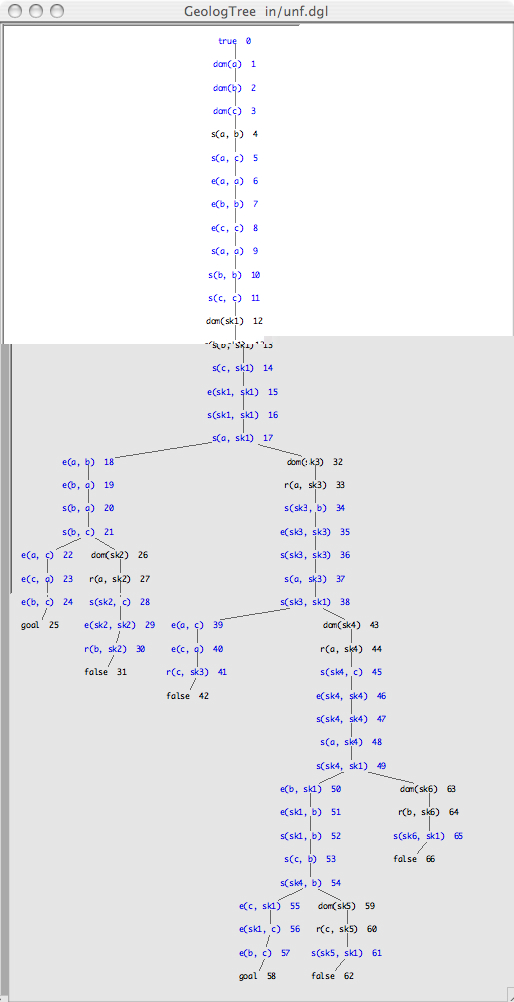
The branch of this proof tree starting at the root and terminating at node #58 is an example of a case proof. There are 6 cases displayed in the diagram. More precisely, the set of Geolog rules used to produce a branch is actually the case proof. Here is a listing of those rules. The rules that the Geoprolog search engine actually used to produce this case (to leaf #58) of the proof are listed next.
Leaf 58:
0, (true=>dom(a))
1, (true=>dom(b))
2, (true=>dom(c))
3, (true=>s(a, b), s(a, c))
5, (dom(a)=>e(a, a))
6, (dom(b)=>e(b, b))
7, (dom(c)=>e(c, c))
8, (e(a, a)=>s(a, a))
9, (e(b, b)=>s(b, b))
10, (e(c, c)=>s(c, c))
11, (s(a, b), s(a, c)=>_G435^ (dom(_G435), s(b, _G435), s(c, _G435)))
14, (dom(sk1)=>e(sk1, sk1))
15, (e(sk1, sk1)=>s(sk1, sk1))
16, (s(a, b), s(b, sk1)=>s(a, sk1))
17, (s(a, b)=>e(a, b);_G520^ (dom(_G520), r(a, _G520), s(_G520, b)))
34, (dom(sk3)=>e(sk3, sk3))
35, (e(sk3, sk3)=>s(sk3, sk3))
36, (r(a, sk3)=>s(a, sk3))
37, (s(sk3, b), s(b, sk1)=>s(sk3, sk1))
38, (s(a, c)=>e(a, c);_G620^ (dom(_G620), r(a, _G620), s(_G620, c)))
45, (dom(sk4)=>e(sk4, sk4))
46, (e(sk4, sk4)=>s(sk4, sk4))
47, (r(a, sk4)=>s(a, sk4))
48, (s(sk4, c), s(c, sk1)=>s(sk4, sk1))
49, (s(b, sk1)=>e(b, sk1);_G720^ (dom(_G720), r(b, _G720), s(_G720, sk1)))
50, (e(b, sk1)=>e(sk1, b))
51, (e(sk1, b)=>s(sk1, b))
52, (s(c, sk1), s(sk1, b)=>s(c, b))
53, (s(sk4, c), s(c, b)=>s(sk4, b))
54, (s(c, sk1)=>e(c, sk1);_G827^ (dom(_G827), r(c, _G827), s(_G827, sk1)))
55, (e(c, sk1)=>e(sk1, c))
56, (e(b, sk1), e(sk1, c)=>e(b, c))
57, (e(b, c)=>goal)
However, this proof is not minimal. The following is a minimal case proof for this case. (Only 7 of the 53 rule applications are needed!)
Notice that the consequents of the applied rules corresponding to facts #49 and #54 are relativized (to the case being proved) for the minimal case proof.Leaf 58: 3, (true=>s(a, b), s(a, c)) 11, (s(a, b), s(a, c)=>dom(sk1), s(b, sk1), s(c, sk1)) 49, (s(b, sk1)=>e(b, sk1)) 54, (s(c, sk1)=>e(c, sk1)) 55, (e(c, sk1)=>e(sk1, c)) 56, (e(b, sk1), e(sk1, c)=>e(b, c)) 57, (e(b, c)=>goal)
It is fairly easy to check that the second listing is a case proof: Read the rules from top to bottom and add facts as they are produced by the rules ... until the last rule produces goal (or false). The proof is minimal because no rule in the sequence can be deleted and still have a proof!
Geoprolog computes minimal case proof using the ?- proof. goal.
?- compile('in/unf').
%% in/unf.in converted to in/unf.gl
true=>dom(a). %1
true=>dom(b). %2
true=>dom(c). %3
e(b, c)=>goal. %4
true=>s(a, b), s(a, c). %5
r(b, _G372)=>false. %6
r(c, _G372)=>false. %7
dom(_G371)=>e(_G371, _G371). %8
e(_G371, _G372)=>e(_G372, _G371). %9
e(_G371, _G372), e(_G372, _G375)=>e(_G371, _G375). %10
e(_G371, _G372), r(_G372, _G375)=>r(_G371, _G375). %11
e(_G371, _G372)=>s(_G371, _G372). %12
r(_G371, _G372)=>s(_G371, _G372). %13
s(_G371, _G372), s(_G372, _G375)=>s(_G371, _G375). %14
s(_G371, _G372), s(_G371, _G375)=>_G493^ (dom(_G493), s(_G372, _G493), s(_G375, _G493)). %15
s(_G371, _G372)=>e(_G371, _G372);_G511^ (dom(_G511), r(_G371, _G511), s(_G511, _G372)). %16
%% in/unf.gl compiled to Prolog.

Yes
?- golog.
Thinking ...
%% in/unf.log created

Yes
?- proof.
Thinking ...
%% in/unf.prf created

Yes
Click of the last link to view the minimal case proof for unf
generated by Geoprolog. Although each case proof in minimal, there is
no assurance, in general, that the proof uses the fewest possible
number of cases.
Exercise: Study minimal case proofs for the examples §6a - §6f.
In order to run the iG system, the reader needs to download the Prolog interpreter iG.pl. The name "iG" is, of course, short for "interactive Geolog". Also, be sure that you have a recent version of GeologTree.jar. The new version of GeologTree.jar is still compatible with the uses described in the previous sections, but the new version also archives a Java GUI that works with iG. Prolog and Java iG programs simply talk to each other via streams over a port on the local system. There is no exchange of objects, only simple text messages.
As an example, consider the following Prolog session. Assume that the session is started from a working directory which contains iG.pl and GeologTree.jar and relevant Geolog theory files ...
?- [iG].

%%%%%%%%%%%%%%%%%%%%%%%%%%%%%%%%%%%%%%%%%%%%%%%%%%%%%%%% 06/7/2007
%%  interactive Geolog
%%   ?- compile(+G).  % Compile Geolog rules in file G.gl
%%   ?- show.         % Show ordered rules ...
%%   ?- iG.           % Start interactive Geolog proof browser ...
%%   ?- info.         % Display this info
%%   ?- more.         % More info about ?-compile(+G). ?-iG.
%%%%%%%%%%%%%%%%%%%%%%%%%%%%%%%%%%%%%%%%%%%%%%%%%%%%%%%%%%%%%%%%%%%

% iG compiled 0.00 sec, 24,832 bytes

Yes
?- compile(dpe).
true=>dom(a). %1
true=>dom(b). %2
true=>dom(c). %3
true=>re(a, b), re(a, c). %4
re(b, _G340), re(c, _G340)=>goal. %5
dom(_G339)=>e(_G339, _G339). %6
e(_G339, _G340)=>e(_G340, _G339). %7
e(_G339, _G340), re(_G340, _G343)=>re(_G339, _G343). %8
e(_G339, _G340)=>re(_G339, _G340). %9
r(_G339, _G340)=>re(_G339, _G340). %10
re(_G339, _G340)=>e(_G339, _G340);r(_G339, _G340). %11
r(_G339, _G340), r(_G339, _G343)=>_G398^ (dom(_G398), r(_G340, _G398), r(_G343, _G398)). %12
%% dpe.gl compiled.

Yes
?- more.
%%%%%%%%%%%%%%%%%%%%%%%%%%%%%%%%%%%%%%%%%%%%%%%%%%%%%%%%%%%%%%%%%%%%
%%  For example, if the Prolog working directory contains a file
%%  ./in/dpe.in then compile it using ?-compile('in/dpe').
%%  If the goal ?-iG. reports errors or hangs, close the Java
%%  window and try again.  Once the Java GUI is ready click
%%  on the "iG?" button for more information about interactions.
%%%%%%%%%%%%%%%%%%%%%%%%%%%%%%%%%%%%%%%%%%%%%%%%%%%%%%%%%%%%%%%%%%%%


Yes
?- iG.
 CLOSE the Java iG window when finished ...
 If connection fails, close Java window
 and try ?-iG. again ...

Spawning Transducer for 1
Spawning Transducer for 2
disable#<=#<=
rule#1#true=>dom(a)
...
The Java GUI will look somthing like the following screen snapshot.
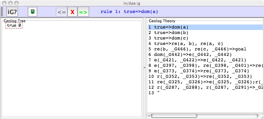
The "iG?" button on the toolbar elicits a help window which shows the following information ...
The following snapshot shows how the tree has developed after several inference steps.The panels
The left pane Geolog Tree displays the active proof search tree. The right pane Geolog Theory shows the Geolog rules and highlights an applicable rule.Infer Button =>
To accepted the selected applicable rule and to extend the proof tree using this applicable rule in the tree window, hit the => button.Block Inference ButtonX
Applicable rules are selected in a top-down fashion. The first applicable rule for the current search tree will initially be selected in the theory panel. To block the application of the selected rule hit the X button on the toolbar. The next applicable rule, if any, will then be selected. Repeatly hitting X will cycle through all applicable rules from top-to-bottom, and then cycle back to top again.Undo Inference Button <=
To undo the last rule application hit the <= button on the toolbar.If there is no applicable rule (indicated by no rule being selected), then try hitting the <= button.
Focus
The focus is the current fact in the tree. The ancestors of the focus in the tree determine the currently applicable rules. The focus is always outlined in red.Inference nodes
Click the mouse on any fact in the tree. If the fact was an inference node (its ancestors satisfied some rule) then the applicable rule will appear in a popup window. Inference nodes are colored blue in the tree.Tree scale
Right-click the mouse on the Geolog Tree pane to popup a scaling menu.Save Geolog tree
The current search tree can be saved at any time. A file dialog will appear. The saved tree can be viewed using the GeologTree jar-application.
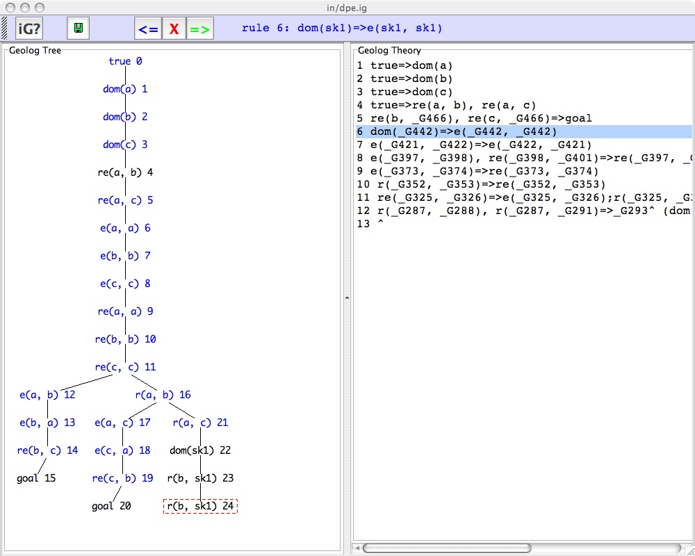
NOTE: Double-click on the (new) Geologtree.jar icon and a Geolog Tree viewer will open...

Drag and drop a tree file (.dgl created by geoprolog or any saved iG tree), in order to view the tree.
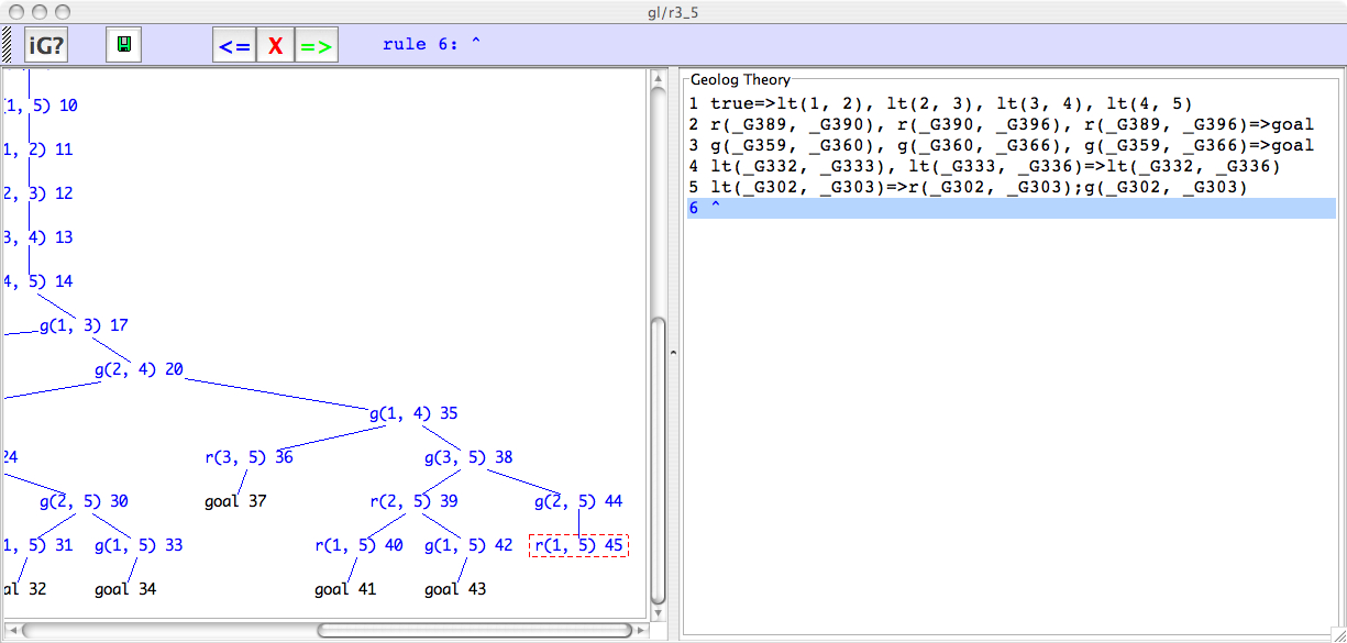
Exercise: Run iG on this example and extract the coloring that produces a countermodel. Draw a picture of this countermodel. Answer.
This current posting for the iG system is a prototype. Check back later for more information and improvements.